
Machine learning for IBNR
Choosing reserving
methods by how well
they predict
Several methods, and many reasonable ways to apply each, give different reserves for the same triangle. The development that would settle the choice has not happened yet.
Learn how machine learning uses past claims development to test familiar methods for IBNR reserving in property and casualty (P&C), or non-life, insurance.
This guide explains published research. The paper is not ReserveAI: its out-of-time AvE and CDR concepts are stepping stones to a much broader platform. See what ReserveAI adds.
Start with the example Read the executive summaryThe orange diagonal is the next period to forecast.
Executive summary
What a chief actuary needs to know
The opportunity is a more consistent, evidence-based way to select reserving methods. Familiar actuarial techniques remain at the centre; historical prediction provides a repeatable basis for choosing how to apply them.
- Make method selection repeatable
- Treat the method and its assumptions as candidates to be tested. Replay earlier valuations using only information available then, score each candidate’s subsequent predictions, and use those scores to inform today’s selection. This makes the reasons for a choice easier to compare, document and challenge.
- Agree what success means
- Actual versus expected (AvE) measures next-period prediction error. The claims development result (CDR) measures the revision in estimated ultimate claims. They can select different methods. Decide which outcome matters for the portfolio, and review both: a stable ultimate estimate can still be wrong.See AvE and CDR explained
- Use the evidence in context
- The paper tests three triangles. Some selections improve ultimate-claims prediction; others make little difference or perform worse. The results support testing this approach on your own portfolio. They do not establish a universal best method or quantify a capital release, reserve reduction or operating-cost saving.
- Keep actuarial judgement central
- The actuary still owns the data, candidate assumptions and final reserve. Changes in inflation, claims handling or business mix can weaken the relevance of historical scores. Review those changes, investigate material differences from the current approach, and record the reasons for any override.
A reserve is also
a prediction
Depending on the method, choices include the history used for development factors, the loss-ratio assumption and how much credibility to give the data. Each choice changes what the method expects to happen next.
We can test those choices by replaying earlier valuations. Fit using only the information available at the time, freeze the prediction, then compare it with the claims development that followed. This is out-of-time validation.
Forecasting the next diagonal
before it is known
The example below fits a chosen method to the known cells of a triangle, freezes its forecast for the next diagonal, and then reveals what was actually observed. Nothing from the future goes into the fit.
Cumulative paid claims · illustrative units. Cells beyond the valuation date are hidden from fitting.
The unknown
next diagonal
The chosen method is fitted to the teal cells, and its predictions for the next period are outlined in orange. These predictions are now frozen.
Changing the method restarts the example.
Inspect the calculation and assumptions
Scores use the paper's absolute-increment-weighted RMSE, across the same existing origin periods. The signed total is shown separately; it is not the RMSE. Development ages with no observed pairs use a factor of 1 in this teaching implementation. There is no added tail beyond the final displayed age.
| Origin | Expected | Actual | AvE | CDR after refit |
|---|---|---|---|---|
| 2017 | 0.00 | Hidden | — | — |
| 2018 | 7.90 | Hidden | — | — |
| 2019 | 16.00 | Hidden | — | — |
| 2020 | 35.46 | Hidden | — | — |
| 2021 | 78.34 | Hidden | — | — |
Machine learning applied
to method selection
Chain Ladder, Bornhuetter–Ferguson and Generalised Cape Cod remain recognisable. Machine learning gives us a systematic way to choose between their many possible applications.
Read about the three methodsThe choices behind a candidate
A method, a history window and a loss-ratio assumption together define one candidate.
The same test for every candidate
Earlier valuations are replayed, and each candidate predicts the next diagonal before it is revealed.
A choice made on the historical scores
The historical scores are compared, and the selected method is then checked against the development that came later.
AvE & CDR · A year in the life of a reserve
The year that happened.
The future we now expect.
A new diagonal tells us what happened. It also changes what we expect to happen next. AvE isolates the first effect. CDR brings both into the same result.
Did this year’s claims match our forecast?
Compare the new experience with the prediction frozen at the previous valuation.
How has the total estimated cost changed?
Include both the new experience and the revised estimate of everything still to come.
- 01 · At the opening valuationFreeze the forecast
Split the reserve into what is expected next year and what is expected after that.
- 02 · Over the next yearObserve the payments
The difference from the frozen next-year forecast is the AvE deviation.
- 03 · At the closing valuationRe-estimate the remaining claims
Use the enlarged triangle to revise the future outlook for those same accident years.
Two questions about one year of development
An illustrative paid-claims example, in undiscounted claims units. Track the same prior accident years at both valuations; exclude the new accident year.
Earlier payments are common to both valuations, so they cancel. Compare the opening reserve with payments plus the closing reserve, not with the closing reserve alone.
Change payments, then change the future estimate. These controls isolate the arithmetic; they are not fitting a reserving model.
The bridge below uses this guide’s sign: positive CDR means a higher ultimate.
The signed components offset: +6 and −10 combine to −4. Square -4 when scoring CDR, not the two components separately.
The total estimated cost falls by 4. That movement includes the payment surprise and the change in the future outlook.
Same development. Two sign conventions.
Switch the convention. The underlying claims and the economic outcome stay the same.
Favourable developmentPrevious ultimate − revised ultimate
Merz–Wüthrich: observable CDR, Definition 2.5, equation (2.19), printed page 552. This guide follows the opposite sign in Balona–Richman §2.2. AvE here remains actual minus expected, in claims units rather than a ratio.
The one-year insight
One year of learning can change many years of claims.
Merz and Wüthrich’s 2008 paper studies the change between successive ultimate estimates. A one-year view includes the revaluation of the remaining run-off, even when settlement is many years away.
Read the two signals together
A quiet CDR can hide a noisy year.
Higher payments can be offset by a lower future estimate. Or payments can match the forecast while the future estimate rises. Check the components before interpreting a small total as evidence of a good forecast.
From a realised CDR to one-year reserve risk
After the year, CDR is an observed result. Before the year, it is uncertain. Under distribution-free chain-ladder assumptions, Merz and Wüthrich estimate the conditional mean squared error of predicting the observable CDR by zero.
That prospective MSEP differs from the historical weighted RMSE used to select candidates in this guide. A realised CDR, or its square, is not by itself a capital requirement or a full predictive distribution.
Read §3, equation (3.1) · printed page 554Results on
three published triangles
The paper tests selection on three triangles with different development patterns and levels of volatility. In some cases selection reduced the error of the forecast ultimate, and in others it made little difference or made the forecast worse. Both kinds of result are shown below.
Both selections gave a lower RMSE than the baseline
AvE-selected BF improves ultimate RMSE by 19.5%; CDR-selected BF improves it by 8.8%.
Read the reported values and their scope
These are transcribed paper results, not outputs from this website's replay. RMSE is measured against the paper's final development values, in source triangle units. A smaller reserve is not itself a better prediction.
| Selection | Method | Ultimate RMSE | Change from baseline |
|---|---|---|---|
| Basic GCC | GCC | 3,170.88 | 0.00% |
| Selected by AvE | BF | 2,552.39 | −19.51% |
| Selected by CDR | BF | 2,893.23 | −8.76% |
Source Balona and Richman (2021) manuscript, table lt_tuning_scores. How this site uses the paper
The guide
in seven chapters
The chapters can be read in order, or entered at the one that answers a particular question. Each chapter gives the intuition, the calculation and the passage of the paper it rests on.
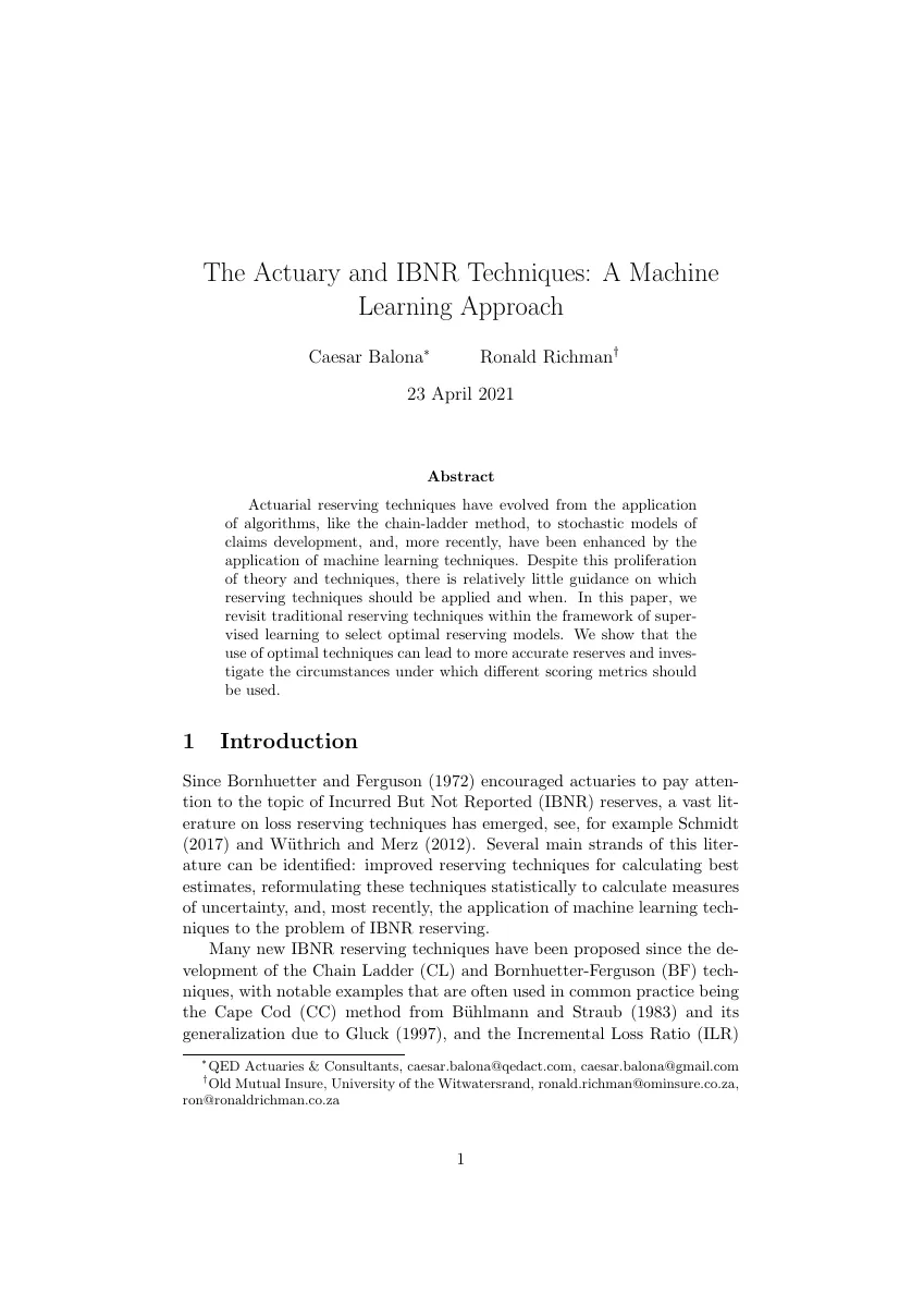
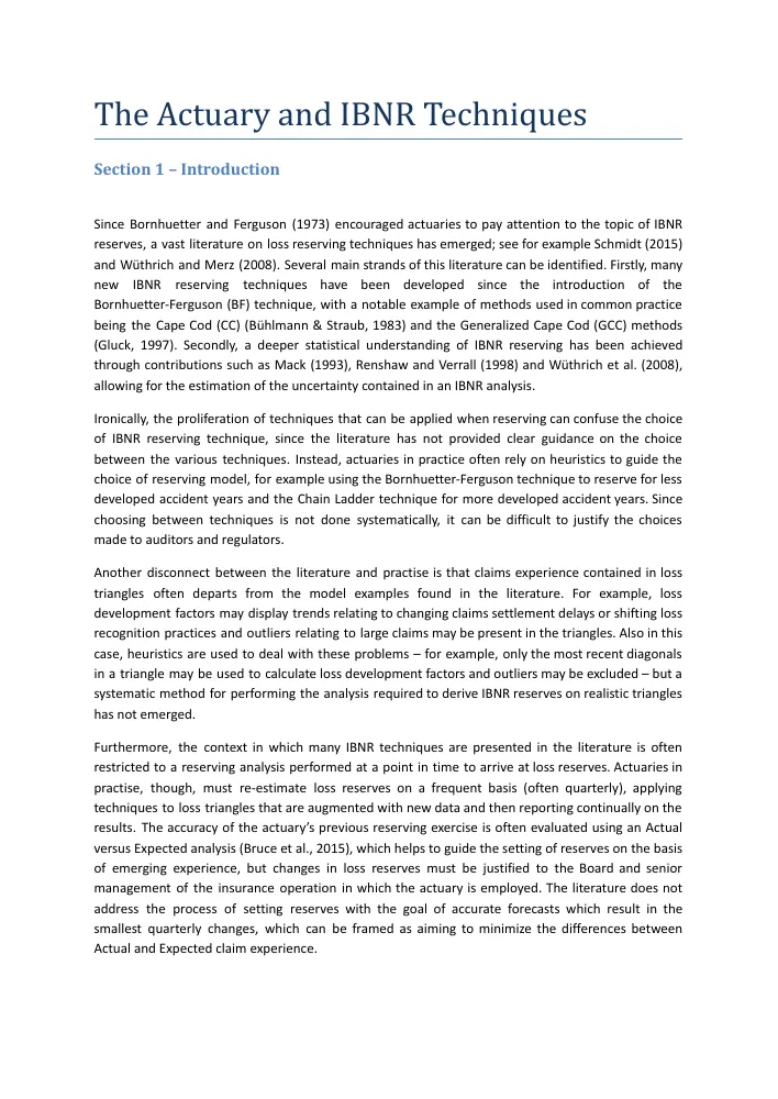 Open the original
 Before the full paper
The early draft
The early draft puts the question plainly: with so many reserving techniques available, how should an actuary choose? Its answer begins with replaying earlier decisions and examining the experience that followed.
The idea dates to 2017. The early draft is undated; the paper is the joint work of Caesar Balona and Ronald Richman.
Making machine-learning reserving
work in practice.
The principle is published. The practical advantage is built into ReserveAI.
ReserveAI’s patent-pending technology makes these ideas work in day-to-day reserving. Our additions are central to the methodology and dramatically improve its practical usefulness.
Discover ReserveAI